365 Days of Climate Awareness 322 – General circulation models 3: boundary conditions

I’ll admit that the term “boundary conditions” used to make me twitch. Partial differential equations and 4-dimensional (three physical dimensions plus time) calculus were always difficult hurdles for me (and not a small part of the reason why I moved from physics over to geology!) But differential equations—diffEQ’s, as they’re known in the biz—are the real mathematic sorcery within climate, or almost any natural system model. In the end, you plug numbers into the many different variables and receive numerical output. You can look at all math as just increasingly fancy types of addition and subtraction. But what makes an equation “differential” is that it focuses on differences.

A sine wave, broken into a series of discrete measurements. 

This is because a “differential” in mathematics is computed from a rate of change. How much does one variable (y, for example) change when another (x) changes? This rate of change itself can vary: an increase in (x) of 1 might under different circumstances produce different changes in (y). Look at the sine wave, a smoothly varying curve, in the illustration. With each identical forward step in the horizontal axis (x), the height (y) changes by a slightly different amount from the previous, and following, amounts. That’s what creates the curve, as opposed to a straight line. In a curve, the rate of change—the slope of the graph—changes as you move along it. That’s bad enough. How about more variables? What if (y) depends not only on (x), but also on (z), (a) and (b)? Hence the sorcery!

Ye olde diffEQ. The differential proper: dy ("change in y") over ("with respect to") dx ("change in x"). Not a constant! Change in the differential's value is the heart of mathematical modeling.

In nature, where just about nothing is constant (though we often pretend they are, to simplify the math), rates of change are the simplest means to approach almost any topic. Predicting the water level and current velocity of tides—extremely important for shipping—are an ideal application of diffEQ’s. Disease control, where microbes grow exponentially—with increasing speed as their population grows, until the system becomes full—is another. For a climate example, the temperature of ocean water will vary in space—east (x), north (y), depth (z), and in time (t). Those four fundamental variables determine quite a lot, but not everything!

Exponential increase in global COVID cases, early 2020.

But nature also has limits. COVID did not continue to spread unchecked, because earth’s population is finite, and the spread rate decreased, and (much) later the actual case load began to decrease. A cycle like the tides has inherent limits within itself—the regular motion of earth and moon—but their height and flow rates are also constrained by things such as the local bathymetry, which limit how much water can pass through. These natural limits, whether based on population, physical barriers like mountains or coastlines, or physical properties like wind speed or incoming solar radiation, are called boundary conditions.

Measurements of tidal height (red) and current (blue) for the St. John's River in Jacksonville, FL Note that the curves are slightly out of phase. The cycle of tidal height lags slightly behind the cycle of current speed.

A more complex species of diffEQ’s contains these built-in boundaries, so the system and its variables don’t become unrealistic. This is because climate models are relentlessly tuned to known, measured aspects of global climate. In climate models, most boundary conditions are empirical: that is, based on measurements, not theoretical derivations. Topography (mountains, valleys, plains.) and bathymetry (coastlines, channels and basins) are two obvious, measured boundary conditions. Other empirical boundary conditions include the amount of solar energy entering earth’s climate system (not constant! Because earth is in motion, and its orbit is elliptical), changing land use patterns (a very important aspect), and many more. These models are complicated.

Tomorrow: some of the main boundary conditions used in IPCC climate models.

Be brave, be steadfast, and be well.

365 Days of Climate Awareness 321 – General Circulation Models 2: basic concepts of flow

Climate models must mimic the observed data. Using the basic fluid dynamics equations (Navier-Stokes and continuity) as a foundation, models attempt to reproduce, in simplified form, not only the basic patterns we have observed, but shorter-term variations. This type of resolution in time and space gives the models enough fidelity to reality to then model long-term trends, over timescales of a century or more.

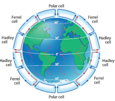
Global wind circulation cells.

In an earlier post (#38, Global Wind Circulation Cells) we looked at the combined influence of uneven heating between equator and poles and the earth’s rotation to produce a series of bands, segregated by latitude, of easterly (from the east) and westerly (from the west) winds. The story of global climate starts here, because even though the ocean contains more than twenty times as much heat as the atmosphere, the bulk of ocean currents are wind-driven, and winds are driven by uneven heating across the earth. The wind-driven currents, like the Gulf Stream and North Atlantic Current, set up the thermohaline (density-driven, vertical) currents where warm water evaporates and the resulting, cooler ocean water sinks.

What you might think wind patterns would make the ocean do (left), versus what happens when you include the Coriolis effect distorting the gyre: western intensification.

A fundamental characteristic of ocean currents is that they tend to be narrower and more intense on the western edge of the ocean basin, but slower and broader on the eastern side. This is due to the combined effects of the Hadley (tropical, easterly) and Ferrel (subtropical, westerly) wind cells which combine to create major ocean gyres around the world. The ocean water, pushed against a continent like North America by the easterly trade winds, is then forced north (to the right) by the combined influence of the Coriolis effect and the continent blocking westward flow.

General concept of the ocean circulation system.

The Coriolis effect gains strength as you move away from the Equator and toward the poles. So the westerly (Ferrel cell) winds, being at a higher (more poleward) latitude than the tropical trades, push the water harder to the south (right). The eastward portion of the wind-driven ocean current acquires a more gently, consistently southward bend and the overall ocean gyre takes on an imbalanced look. The westward, tropical arm of the gyre is driven into the continental shelf, where it is diverted poleward by the shallowing land mass.

Any general circulation model, the type used for climate simulations over the course of years or decades, begins with these basic concepts: the latitude-constrained wind cells, and the wind-driven ocean gyres which are intensified on the western edge when bordering a continent. Together they constitute a “first-order approximation”, that is, a general but inaccurate model which needs to be tuned with more specific information.

Tomorrow: Adding detail to a climate model.

Be brave, be steadfast, and be well.

365 Days of Climate Awareness 320 – General Circulation Models 1: Introduction

A fluid is any state of matter where the atoms or molecules do not stay in fixed spatial relationships with their neighbors. This includes liquid, gaseous and plasma states. We’re not worried about plasma because that occurs only at extremely high temperatures, like in the sun. On earth we deal with liquid and gas. Fluid dynamics deals with the motion and energy states of any fluid, and computational fluid dynamics is the computerized version of this. Geophysical fluid dynamics is a specific sub-branch of fluid dynamics.

Hydrodynamic model of a ship's hull moving through the water.

There are many different types of fluid dynamics models, including within earth sciences! Testing and computer modeling are used in conjunction to analyze the performance of machines and of natural systems, including rivers, ship hulls airplane wings, and many, many more. But to be a properly geophysical in nature, a flow of air or water must meet three conditions:1)       

Aerodynamic model of a plane wing.

Fluid dyamic model (but not geophysical) of a channel and lagoon.

 1) It occurs on a sphere (or, more properly, an oblate spheroid, since the earth bulges a little around the equator);

2)         2) The sphere is rotating, which affects the fluid’s motion;

3)        3) The aspect ratio of the fluid is extremely thin. For example, the Atlantic ocean is roughly 4 km deep and 4,000 km across, for a very approximate aspect ratio of 1:1000, not unlike that of the edge of a piece of paper.

The planet's rotation, with different velocities at different latitudes.

Approximate aspect ratio of the Atlantic Ocean (with earth's curvature included).

These three conditions impose severe limitations on the types of motion the fluid is likely to undergo, with resulting effects on the equations (not touching those here! And it’s been years since I’ve tried to knock any rust off my math skills). The main effects of these conditions is to limit the ocean and atmosphere—we’re not going to worry about the mantle or core, which are separate cases—to mostly stratified, horizontal motions, with limited convection and a strong Coriolis (rotational) component. This branch is the domain of climate modelers.

Tomorrow: General circulation models 2: basic components of flow

Be brave, be steadfast, and be well.

365 Days of Climate Awareness 319 – Global Warming Potential

Global warming potential (GWP) is the analytical method for comparing different greenhouse gases. They differ both in their absorptive capacity, known as “radiative efficiency”, and in their residence time, known as lifetime, in the atmosphere. The combination of those two yields the gas’ total potential for warming the planet. In these calculations as in other measures, water vapor, itself a very powerful greenhouse gas, is not included because it is not considered “well-mixed”. That is to say, concentrations of H₂O vapor vary very widely in time and space around the world due to weather and climatic conditions.

Atmospheric concentration of carbon dioxide.

Global warming potential is treated as a scalar: that is to say, a number without units, because all greenhouse gases are compared to carbon dioxide. CO₂, by definition, has a GWP of 1. Since the gases have vastly different lifetimes: carbon dioxide, roughly 120 years, methane roughly 10.4, and CFCs less than that, their warming potential is averaged into a 100-year span. A few principle gases, using this 100-year average, are listed below. (For concentrations: ppm = parts per million; ppb = parts per billion; ppt = parts per trillion.)

1)     

Atmospheric concentration of methane.

1)  Carbon dioxide (CO₂): GWP = 1; lifetime ~120 yrs (but can vary widely); 410 ppm

2)      2) Methane (CH₄): GWP = 28; lifetime = 10.5 yrs; 1,800 ppb

3)      3) Nitrous oxide (N₂O): GWP = 265; lifetime = 132 yrs; 380 ppb

4)      4) Various chlorofluorocarbons (CFCs): 4,660-13,900; lifetimes 16-500 yrs; 1-100 ppt

5)      5) Sulfur hexafluoride (SF₆): GWP = 23,500; lifetime = 3,200 yrs; 10 ppt

Atmospheric concentration of nitrous oxide.

Different time frames (20 years, 200 years) are used by different agencies around the world, but the concept is the same: amount of energy absorbed by a given mass of greenhouse gas during that time, given the average solar input of roughly 1.366 kW/sq m. With this statistical tool scientists can directly compare the impacts of various gases, though for high-resolution climate modeling, the different gases with their distinct behaviors are accounted for separately.

Atmospheric concentrations of fluorocarbons and other chemicals.

Tomorrow: introduction to general circulation models.

Be brave, be steadfast, and be well.

365 Days of Climate Awareness 318 – Global Overview of Emissions and Warming

con

Emissions of carbon dioxide and carbon dioxide equivalent continue to rise globally. Carbon dioxide equivalent is the modeled sum of CO₂ and non-CO₂ greenhouse gases including methane, sulfur hexafluoride (SF₆)  and others. It is a more complicated concept since the gases do not have equivalent behaviors or residence times in the atmosphere. Direct measurements of the gases in question are translated into warming potentials and so folded into modeling calculations.

Global CO₂ concentration vs temperature rise.

Actual and projected emissions vs temperature rise relative to 1.5-degree increase goal.

The measurements show that declining absolute and per-capita emissions from the richer countries on earth show declining emissions in recent years which is overwhelmed by the developing world. Even as improvements in efficiency and renewable capacity provide some hope in the climate situation, the planet’s economic momentum tells the opposite story. Poor and developing countries point out rightly that they especially, in geographically disadvantaged positions, are paying the highest environmental and social tolls for the problem which the industrialized world created.

Annual CO₂  emissions by economic stratum.

Cumulative CO₂  emissions by economic stratum.

But it’s more than a problem of justice. It’s also an issue of human nature itself, of individuals’ and groups’ collective desires to improve their circumstances, in this case with economic tools of proven destructiveness. Albert Einstein’s famous quote can be applied perfectly here: “We cannot solve our problems with the same thinking we used when we created them.” The delusion that the planet can continue growing economically and commit itself to always-greater material prosperity is one of the greatest hurdles we face.

Per capita CO₂  emissions by economic stratum.

Tomorrow: global warming potentials.

Be brave, be steadfast, and be well.

365 Days of Climate Awareness 317 – China and Climate Change

China’s climate ranges from tropical in its extreme south, to subtropical and monsoonal, to cold and dry in the north, though the bulk of its heartland is temperate. Broadly, global warming will have a disproportionate effect in China’s north, where winters will become milder and summers longer and warmer. Over the past 60 years, China has seen an increase in average temperatures throughout the country, including central and south. Bucking the global trend, however, there has been a 50% decrease in extreme events like floods, droughts and severe storms, correlated with the weakening of the East Asian monsoon.

Köppen-Geiger climate zones, 1980-2016

Predicted Köppen-Geiger climate zones, 2071-2100

Sea level rise along China’s coast has been averaging 3.4 mm/0.13 in per year since 1980, giving an average increase of 7.5 cm/2.9 in in that time. Some areas, such as Hong Kong, have seen seal level rise of more than 10 cm. While harbors such as Shanghai, 3 m/9.8 ft above sea level, are not in imminent danger of being inundated, sea level rise does heighten the risk of catastrophic storm flooding.

Temperature anomaly in China.

Climate Action report card.

Agriculture in China has already suffered, and will suffer further with increasingly violent rain in the south, and decreasing rain levels in the north, as the tropical zone becomes wetter and the subtropical and temperate zones become more arid. At the same time, higher temperatures are likely to increase disease and pest infestation rates, lowering productivity.

Mid-20th century summer East Asian monsoon (left); current, weakening summer East Asian monsoon (right).

Modeled changes in 21st century drought index: decrease - drier; increase = wetter.

Increasing temperature and acidity in the oceans is putting major ecosystems like coral reefs in the South China Sea under severe stress, and lowering fish populations throughout the region. Combined with overfishing—China’s fishing fleet is considered one of the world’s worst offenders at poaching, as they pursue fishing grounds to augment their own—ocean productivity has been declining for several decades, and is likely to decline further.

Tomorrow: overview of climate change’s global impact.

Be brave, and be well. Especially now.

365 Days of Climate Awareness 316 – Major global CO2 emissions

This post began as “Carbon emissions of China”, but that seemed to me too limited (despite these posts’ brevity) because of the predictable, repeated, pattern: increasing annual and cumulative CO₂ emissions as a function of economic activity (excepting the COVID dip). The most encouraging data trends are relative: decreasing carbon intensity in power generation (and overall GDP) and per-capita emissions in many leading economies. The United States and Europe have seen a slight decrease in carbon emissions over the past several years. These decreases, however, are more than overwhelmed by the added emissions of developing countries who want the same benefits of wealth which those already industrialized have.

Annual CO₂ emissions: China, US, EU, India & the world.

Despite legitimate progress in efficiency and in renewable energy capacity, human society remains on a runaway track toward self-destruction due to global warming. The feeble pledges associated with the Paris Agreement’s goal of 1.5°C/2.7°F or less global temperature rise by 2050—with the first global stocktake of greenhouse gas emissions delayed by COVID until 2023—seem unlikely to accomplish much in the face of an unwavering commitment to economic growth.

Per capita CO₂ emissions: China, US, EU, India & the world.

Such strides as China has taken in deploying renewable generation capacity are possible only in an authoritarian society such as theirs. Were there a gorge suitable to trap the Mississippi River in a gigantic reservoir and increase the US’ hydropower by nearly half, there is no way 13 cities and 1.4 million people would be forcibly moved to enable it. The United States’ offshore wind “revolution” has it lagging badly behind other countries with economies a fraction of its size, whereas China has leapfrogged the entire world in the past four years.  It is the motive for individual profit which is the foundation of Western capitalism, and has led to the exploitation of whole populations and the planet itself.

Cumulative CO₂ emissions: China, US, EU, India & the world.

The cultural roots for these differences are profound and unlikely to change. Speaking geopolitically, since the dawn of history China has had a huge population, an estimated 57 million in year 1 CE, roughly a quarter of the world’s total estimated 232 million. In a country first of warring kingdoms and later an empire hemmed in by enemies to south and especially to the north, securing a stable existence for the population was a ruler’s first concern. That primary motive still obtains today, evidenced by China’s steady, almost inexorable pursuit of global economic resources and the military capability to preserve access to them.

Coal-fueled CO₂ emissions: China, US, EU, India & the world.

It is visible in China’s 1949 annexation of Tibet, known as “China’s water tower”, the plateau north of the Himalaya. Much like Israel’s 1967 capture of the Golan Heights, also a regional water source, China secured a vital natural resource as well as a strategic position against its regional opponent, India (or in Israel’s case, Syria). It was a geopolitical act with one goal in mind: securing the livelihood of a giant (1949: 550 million) and growing population.  This was the act of the same country which enacted its (unevenly applied) one-child policy to limit population growth, and now severely limits its people’s access to information and ideas from outside.

Natural gas-fueled CO₂ emissions: China, US, EU, India & the world.

Meanwhile, the United States sprang to life in a geopolitically perfect continent with tremendous natural resources, long coasts with deep ports on two major oceans, a well-connected, navigable internal river system spanning 2/3 of the interior, and a native population which was comparatively easy to sweep aside. An aggressive thirst for growth was baked into the national character very early. As whites spread westward first on foot and later by rail, a sense of the power of the individual and of a national manifest destiny became articles of patriotic faith, and find perhaps their ugliest expression in the “American exceptionalism” of today.

Oil-fueled CO₂ emissions: China, US, EU, India & the world.

The Chinese look at our individual freedoms, our insistence on self-expression and self-fulfillment as anarchistic and globally hazardous. They look at us in the West as refusing to share or intelligently use our resources, the result being an overconsuming, self-indulgent society incapable of correcting itself, and assured of self-destruction. We in turn look at the authoritarian, tightly controlled society of the Chinese as depriving its people of the things that make life most worth living.

Consumption-based CO₂ emissions: China, US, EU, India & the world.

And so we have arrived in the 21^st century, with (broadly) two competing global orders that share a common environmental problem. The next thirty years will likely tell the story of whether we can collectively adapt.

Carbon intensity of electrical power generation: China, US, EU, India & the world.

Tomorrow: effects of climate change in China.

Be brave, and be well.

365 Days of Climate Awareness 315 – China and Rare Earths

The rare earth elements, also known as REEs, rare earth metals or rare earth oxides, are a chemical class of metallic elements known as the lanthanides (plus two others, scandium and yttrium, also in column 3 of the periodic table of elements). The lanthanides are so named due to their similar behavior to lanthanum. In the periodic table, they are the upper row in the subset usually drawn beneath the rest of the chart (drawn this way to keep the chart from being too wide for the page). As in the illustration in this post, the lanthanide series slips in between lanthanum (atomic number 57) and halfnium (72). There are seventeen rare earth elements/lanthanides, and they are critical for much of our developing renewable energy technology. (For a more detailed list of each element and its uses, please refer to the Wikipedia article.)

Periodic table of the elements, standard view

Periodic table, lanthanides and actinides shown in series

Rare earths are not uncommon in Earth’s crust, ranging between 150-220 parts per million (ppm) and one, cerium, being more common than copper (though promethium, a radioactive metal with a half-life of 17.7 years, is in fact extremely rare). The “rare” moniker comes from the fact that these elements are not found in concentrated deposits like most metals such as iron, uranium or gold. When present, they are distributed very sparsely, though several different rare earth elements are often found together (likely due to the similarity in their chemical behaviors). REEs are found both in crustal rock and in the regolith, the weathered sediment lying on top of crustal (bed-) rock.

Global rare earth production.

Rare earth mining in the regolith (sedimentary layer).

Rare-earth elements have several applications in renewable energy technologies (not including photovoltaic cells, which might surprise you). Their main applications are in specialized magnets, as specialized alloys (metallic blends, either as a mixture or a chemical compound), chemical catalysts, and as polishing compounds, and others even more particular. The typical method of mining these is by open pit, where tons of rock are transported to a plant and the REEs are chemically isolated and concentrated. It is a tremendously energy-intensive process which leaves massive scars on the planet surface. There is also the problem of disposing of the waste, the leftovers from chemical solutions used to extract the REEs.

Industrial applications for rare earth elements.

Global rare earth market share through the years.

China has 50% of the world’s currently known deposits of these elements, and is the source of nearly 90% of global production (nearly 150,000 metric tons/165,000 tons in 2019). Since rare earth elements are considered strategic—being hard to find and impossible to replace—China’s overwhelming market position is considered a hazard by governments and markets around the world. Research is underway both to make REE extraction methods less environmentally destructive and to circumvent use of those elements altogether.

Rare earth strip mine in China.

Tomorrow: Global carbon emissions.

Be brave, and be well.